Quantum designs: faster averaging over quantum states and unitaries

Table of Contents

• Introduction
  • Prerequisites
  • Notation
  • Organization of the post
• Tooling
  • Theoretical tools
  • Software tools
• Spherical designs
  • Average of a function over a line
  • Average of a function over a circle
  • Average of a function over a sphere
  • Average of a function over $n$-spheres
• State designs
  • Functions of a quantum state and their average
  • Average of a function over the Bloch sphere: analytic solution
  • Average of a function over the Bloch sphere: Monte Carlo integration
  • Average of a function over the Bloch sphere: state designs
  • Application: average gate fidelity
• Unitary designs
  • Functions of a unitary and their average
  • Average of a function of a unitary: analytic solution
  • Average of a function of a unitary: Monte Carlo integration
  • Average of a function of a unitary: unitary designs
  • Application: average gate fidelity
• Next steps
• Conclusion
• Supplementary material
  • Generating permutation matrices
  • Generating the Pauli group
  • Generating the Clifford group

Introduction

Consider the following problem: given a quantum gate, what is the probability that under noise it fails to evolve a given state the expected way?

Our first step will be to define the quality of implementation of a quantum gate. This is done using the notion of fidelity which measures how close the implemented quantum gate approximates the ideal quantum gate.

The method used to determine the fidelity of a quantum gate can either be quantum process tomography (QPT) or quantum gate set tomography (GST).

The problem with both QPT and GST is that they are expensive to carry out. So an alternative method is to find a large random number of states and see how the implemented gate performs on each of those states compared to the performance of the ideal gate. We then take the average of fidelities over all those states.

But that can also be quite expensive because it will require a large number of states if we want the calculated average to be meaningful.
And that’s where designs enter the picture: by using a small, well-chosen, representative set of states we can calculate the average fidelity without using a large number of samples.

It is our goal in this post to build some intuition about designs, in particular unitary designs, by working through small examples. For the sake of this goal, we won’t dig deep into the mathematics and focus more on the basic principles via illustrative examples and code.

Also quantum designs are used for other things besides calculations of the average fidelity but we will focus on averages to simplify understanding.

Prerequisites

It is assumed the reader can do basic integral calculations and can program in Python.

The reader is also assumed to know basics of quantum computation. We won’t use anything fancy but simple quantum circuits.

Notation

Quantum states can be written in a variety of ways but for computational purposes, we will adopt the trigonometric form since it will be convenient in computing integrals:

We will make use of Pauli matrices:

• Identity $I$ matrix:

• Pauli $X$ matrix:

• Pauli $Y$ matrix:

• Pauli $Z$ matrix:

And of matrices that generate the Clifford group:

• Hadamard gate:

• Phase gate:

Organization of the post

In the next section, we introduce all the tools we need to successfully make use of this post.

The section that follows is on spherical designs: before we touch upon quantum designs, it is fruitful to acquaint ourselves with (classical) spherical designs so that we can appreciate the power of designs in general.

We follow with states designs as a prelude to unitary designs so as to strengthen our intuition about what integration over the Haar measure and quantum designs are about.

Then we explore unitary designs and work through an example where the power of unitary designs come to rescue us from computing complicated integrals and more importantly from performing expensive computations.

We then talk about what we didn’t touch upon and consequently what’s worth learning more about assuming we have come to appreciate the power of designs.

Last we give some concluding remarks.

Tooling

Passing familiarity with Python and Numpy is always assumed on the software side and linear algebra on the theory side.

Theoretical tools

On the mathematics side of things, the following will be useful to know:

• Computing simple simple integrals: when not able or willing, please use Wolfram Alpha.
• Performing matrix and vector operations such as addition and multiplication.

On the quantum computing side of things we will need to know:

• What quantum states and gates are.
• What a quantum channel is.

Software tools

We will use PennyLane from Xanadu to run simulations.

The installation instructions can be found at https://pennylane.ai/install/.

For this post, I used PennyLane==0.32.0, numpy==1.23.5, and scipy==1.11.2.

Spherical designs

Say we want to find the average of some function over a sphere. You might go: wait, why would I want to do that? In general, the problem we are working with will dictate whether we need to use a sphere, a line, a cylinder, etc. In the case of quantum computing, for instance, an ideal qubit can be described geometrically as points on the surface of a sphere, the Bloch sphere. So learning to work with spheres is a good starting point.

(Another example: if we want to compute the average of a function over the earth, assuming the earth is a sphere is a good approximation.)

We will start with a refresher though: computing averages over a line (an interval to be exact). Then we will move to spheres. Note that a circle is also defined as a sphere, a $2$ dimensional one: the $1$-sphere. The sphere we are used to is a $3$ dimensional one, the $2$-sphere. And there are spheres in dimensions more than $3$, we just won’t bother with them.

Average of a function over a line

To get started, as a segue to the fun stuff, let’s compute the average of a simple function over an interval.

This subsection won’t introduce designs but will show a general method of computing averages of functions by using random samples drawn from an interval.

Average of a function over the line

Our mission is to find the average of $f(x) = -x^2+4$ over the interval $[-1, 1]$.

The average of an arbitrary function $f(x)$ over an interval $[a,b]$ is computed using the formula:

Therefore in our case, the average is computed as follows:

Average of a function over a line: Monte Carlo integration

Let us now compute that average using Monte Carlo integration which is a general method for performing numerical integration. The procedure is very simple: uniformly take $N$ samples from the interval $[a, b]$, calculate $f(x)$ for each sample $x$ then divide by the total number of samples. Essentially the same way a normal average is calculated:

Where $x_{i}^{line}$ means that each point $x_i$ is sampled uniformly from some line.

Coding the above formula in Python, we obtain a similar result to the analytical result above:

import numpy as np

def monte_carlo_average(f, a, b, sample_size):
    """Compute the average of a function `f` in the interval [a,b)
    The interval is right-open because of the implementation of
    `np.random.uniform` but it doesn't affect our final result
    because we just need to get arbitrarily close to  `b`.
    """
    if b - a == 0:
        raise ValueError(f"Cannot compute the average in the interval [{a},{b}].")

    return np.mean(np.random.uniform(a, b, sample_size))

if __name__ == "__main__":
    f = lambda x: 4 - x**2
    print(monte_carlo_average(f, -1, 1, 100_000))

In the code above, we used $100000$ samples. The lower the number of samples we use, the farther we get away from the true average. The more samples we use, the longer it takes to obtain the result we seek.

This observation is very important because it forms the justification of using designs as we will quickly see in the following subsections.

Average of a function over a circle

As mentioned before, circles are also spheres but we treat them separately so that our intuition is built in a smooth way, starting with something very simple.

Integration over the circle exhibits all the necessary aspects that will allow us to introduce designs but at the same time it is easy to work with, especially finding analytical solutions.

This is important because as we move to spheres and beyond, it gets more complicated to find analytical solutions.

Area of a circle

To calculate the average, we first need to calculate the area of a circle. More importantly, we get to look at the Jacobian determinant which will allow us to understand the concept of measure.

Let $z = g(x, y)$ be a continuous function over a region $R$ in the $xy$-plane describing a surface. The surface area enclosed by $z$ is given by:

The equation above can be read as taking the sum of all the little areas $dA$. In cartesian coordinates $dA = \,dx\,dy$.

In the case of a circle, the equation is $r^2 = x^2 + y^2$. We can find the area in cartesian coordinates by expressing $y$ in terms of $x$ with:

We can then calculate the integral:

And get $S = \pi r^2$.

A much more elegant method is to move to polar coordinates from the beginning. This involves a change of variables so let’s talk about that.

Let $x = r(v,w)$ and $y = s(v,w)$. Let us assume that the first derivatives of $r$ and $s$ exist and are continuous. Let $J(v,w) = (x,y)$ be a transformation that maps a region $S$ to the region $R$.

Integration by a change of variables is given by:

The transformation $J = \dfrac{\partial(x,y)}{\partial(v,w)}$ is called the Jacobian. It is a linear map that allows us to do the transformation. The quantity $\det J = \left\lvert \dfrac{\partial(x,y)}{\partial(v,w)} \right\rvert$ is called the Jacobian determinant. It quantifies how much the linear transformation affects the area in space.
If you changed a square in cartesian coordinates to polar coordinates, the area will change. The Jacobian determinant measures that change.

This is very important to grasp because not only we will see the same for spheres but also because even when we move to integration over unitary matrices, we will have to take into account the integration measure in order to properly account for change in area/volume.

We won’t go over the detailed calculations of the Jacobian since this is can be found in most books on calculus. The change of variable is given by $x = r\cos\theta$ and $y = r\sin\theta$. The Jacobian is found to be $J(r,\theta) = r$, and since $r \ge 0$ we have $\det J = r$. It follows that $dA = rdrd\theta$.
The new limits of integration are $0 \le r \le R$ for some fixed radius $R$ and $0 \le \theta \le 2\pi$.

Consequently the surface area of the circle is:

Average of a function over a circle

In general, the average of a function $f(x,y)$ over a circle of unknown radius $r$ is given by:

Note that $r$ is the unknown radius of an arbitrary circle while $R$ is the potentially fixed radius once it is known, that is $r \leftarrow R$. What that means is that once we have calculated the average of $f$, it will depend on $R$.

Let us proceed and find the average of $f(x,y) = x^2$.

First, we move to polar coordinates and find $f(\theta, r)$. The circle we’re integrating over has equation $x^2 + y^2 = R^2$ for some to-be-fixed radius $R$. Since $f$ depends only on $x$ the change to polar coordinates implies $x = R\cos\theta$. It follows then that $f(\theta, r) = R^2\cos^2\theta$.

Now, we can calculate the average using the formula above:

If we are integrating over the unit circle ($R = 1$) then the average will be $\bar{f} = \dfrac{1}{2}$. If $R = 2$, then $\bar{f} = \dfrac{2^2}{2} = 2$.

Average of a function over the unit circle

Now assume that we know $R$ from the beginning. Then there is no need to integrate over the radius, it is a constant from the get-go. The function $f(\theta,r)$ no longer depends on $r$ so we denote it by $f(\theta;R)$.
This is exactly the case when we are averaging over the unit circle since we know that $R = 1$.

In that case we can save ourselves the pain of performing a double integral using the formula:

For a sanity check, let’s repeat the calculation above; to find the average of $f(x,y) = x^2$ over the unit circle. Since $R=1$, it follows that $f(\theta; R) = R^2 \cos^2\theta = \cos^2\theta$.

And this matches the result obtained by not fixing $R$ and providing it later.

The advantage of this latter method is that most of the time we already know the radius and for problems we will care about $R=1$ – whence the unit circle.

This is not at all particularly interesting or practically useful, but an important stepping stone that will lead us towards our goal of finding these averages using designs.

Average of a function over the unit circle: Monte Carlo integration

Just as with the line, we need to sample uniformly from the unit circle. The formula itself doesn’t change:

Where $x_{i}^{circle}$ ($y_{i}^{circle}$) means that each $x_i$ ($y_i$) is sampled uniformly from the circle.

To sample uniformly from the circle, we use the circle trigonometric parametrization (Ozols, 2009):

Where $\mathbb{S}^1$ is the 1-sphere (circle).
Uniform sampling simply involves uniformly sampling from the interval $[0, 2\pi)$.

With that said the code is straightforward. So let’s see if for $f(x,y)=x^2$ we do get the average $\bar{f}=\dfrac{1}{2}=0.5$.

import numpy as np

def monte_carlo_average(f, sample_size):
    """Compute the average of a function `f` over the unit circle.
    """
    def sample_from_circle(size):
        theta = np.random.uniform(0, 2 * np.pi, size)
        return zip(
            np.cos(theta),
            np.sin(theta)
        )

    return np.mean([f(*sample) for sample in sample_from_circle(sample_size)])

if __name__ == "__main__":
    f = lambda x, y: x**2
    print(monte_carlo_average(f, 100_000))

We are now in a position to introduce designs, and of course these are going to be circular designs.
Understanding circular designs is going to be enough to appreciate the value they bring to the table!

Circular designs

Using Monte Carlo integration, we’ve been able to calculate the average of some function $f(x,y)$ over the circle. This method requires drawing random (uniform) samples then computing the average the usual way.

With circular designs, under certain conditions, we can find that average by using a set of carefully chosen points depending on the degree of the polynomial that makes the function we wish to average.

We start by defining what a circular design is:

Definition: let $f_t: \mathcal{S}(\mathbb{R}^2) \rightarrow \mathbb{R}$ be a polynomial in $2$ variables homogeneous in degree at most $t$. A set $X = \{ x \vert x \in \mathcal{S}(\mathbb{R}^2) \}$ is a circular $t$-design if:

\[\dfrac{1}{\lvert X \rvert} \sum_{x \in X} f_t(x) = \dfrac{1}{\pi R^2} \int_{0}^{2\pi} \int_{0}^R f_t(\theta, r) r\,dr\,d\theta \tag{6}\]

holds for all possible $f_t$. Moreover a circular $t$-design is also a circular $s$-design for all $0 < s < t$.

Let’s first understand the definition before finding what our circular $t$-designs are:

1. We require that the function $f_t(x,y)$ be a polynomial.
2. The polynomial $f_t$ must be homogeneous in degree at most $t$. This means the sum of each of the degrees of the terms in the polynomial is the same and it is $t$.
3. The set $X$ is finite otherwise calculating $\dfrac{1}{\lvert X \rvert}$ is not possible.
4. Given $s < t$, wherever an $s$-design works, so will a $t$-design.
5. To accurately compute the average of a polynomial of degree $t$, we must use a $t$-design.

Here are a few examples to help understand the definition:

• $f(x,y) = x^2$ is a homogeneous polynomial of degree $2$.
• $f(x, y) = x^2 + y$ is not a homogeneous polynomial: $x^2$ is of degree $2$ while $y$ is of degree $1$..
• $f(x, y) = x^2 + xy$ is a homogeneous polynomial of degree $2$: $x^2$ is of degree $2$ and the sum of degrees in $xy$ is $2$.
• $f(x, y) = x^8 + x^5\,y^3 + x\,y^7$ is a homogeneous polynomial of degree $8$.

So, what are the circular designs we will work with? It has been shown that polygons are circular designs (Bannai & Bannai, 2009), specifically the $(t+1)$-gon is a circular $t$-design.

As examples we have that the digon is a $1$-design, the triangle is a $2$-design, the square a $3$-design, and so on.

Thus if we have a polynomial of degree $5$, we should use a $6$-gon (hexagon) as our $5$-design.

What then are the points we will need to evaluate the polynomial $f(x,y)$ at in order to compute the average we seek? Those are simply the points corresponding to the vertex corners of the polygon.

Without further ado, let’s write some code that computes the average of $f(x,y) = x^8 + x^5\,y^3 + x\,y^7$ using circular t-designs.

import numpy as np

def circular_design_average(f, t):
    """Computes the average of a function `f` using circular
    `t`-designs, specifically polygons.
    """
    def polygon(number_of_sides):
        """
        Given the number of sides, this function returns
        the coordinates of the vertex corners of the polygon with
        the given number of sides.
        """
        internal_angle = 2 * np.pi / number_of_sides
        coordinates = []
        
        for point in range(number_of_sides):
            new_angle = point * internal_angle
            coordinates.append([np.cos(new_angle), np.sin(new_angle)])
        
        return coordinates

    # Calculate the mean of the function evaluated at
    # the vertex corners of the polygon
    return np.mean([f(*point) for point in polygon(t + 1)])

if __name__ == "__main__":
    f = lambda x, y: x**8 + (x**5)*(y**3) + x*(y**7)
    for vertex_count in range(2, 15):
        print(f"Design = {vertex_count - 1}\t\
                average = {circular_design_average(f, vertex_count)}")

It is worth looking at the output of the code above and make some comments:

Design = 2      average = 0.33593749999999994
Design = 3      average = 0.5
Design = 4      average = 0.2734375
Design = 5      average = 0.33593749999999994
Design = 6      average = 0.2734375
Design = 7      average = 0.28125
Design = 8      average = 0.27343749999999994
Design = 9      average = 0.27343749999999994
Design = 10     average = 0.27343750000000006
Design = 11     average = 0.27343749999999994
Design = 12     average = 0.27343749999999994
Design = 13     average = 0.2734375
Design = 14     average = 0.2734374999999999

So what have we learned from the result above?

1. If we tried computing the average analytically (via integration), we would have ended up needing to evaluate integrals with sines and cosines of degree at least $3$, not fun!
2. Using Monte Carlo, we need a large number of samples in order to approximate the average of the function. Using a circular $9$-design, we required only $9$ evaluation of the function. Moreover, because Monte Carlo relies on random sampling, we will not get the same exact result with each run.
3. While we may get the correct result using a $t$-design $t < 8$ (e.g.: $t = 6$), we can’t rely on that. Notice that for $t = 5$, we got the wrong result even though the result was correct for $t = 4$ and $t = 6$.
   But notice how the result remains pretty consistent for $t \ge 8$. And that makes sense: we are just using more points so accuracy should either increase or stay the same.

And that’s pretty much the essence of using designs: approximate function averaging over some set using as few function evaluations as possible.
In the sections that follow, we wil simply introduce new sets over which to measure and new designs to tackle different problems.

Average of a function over a sphere

Averaging over a $2$-sphere is pretty much the same as averaging over the circle. So we won’t go through the exact same motions and just state the results and perform some simple calculations. Then we introduce the designs that work for the $2$-sphere.

Moving forward, we will refer to the $2$-sphere simply as sphere even if mathematically a sphere generally refer to the $n$-sphere.

Volume of a sphere

The move from cartesian coordinates to spherical coordinates is given by:

The region of integration is given by:

The Jacobian determinant of a sphere is given by:

The volume of a sphere is therefore calculated as:

Again, we can appreciate the importance of using the correct measure obtained from the Jacobian determinant allowing us to compute the correct volume of a sphere of radius $R$.

Average of a function over a sphere

Averaging over a sphere is very similar to averaging over a circle. The only change will be the use of a different measure obtained from the Jacobian determinant. Because of that, we will use the volume of the sphere, not its surface area in the general formula.

In general, the average of a function $f(x, y, z)$ over a sphere of unknown radius is given by:

As an example, let us find the average of $f(x,y,z)=x^4$ over a sphere of radius $R$.
Moving from cartesian coordinates to spherical coordinates, $f$ is now given by $f(r,\theta,\phi)=R^4\sin^4\theta\cos^4\phi$.

Evaluating the integral above, we get:

Average of a function over the unit sphere

Same as with the circle, we can make a simplification of the averaging formula if the radius is a known constant. The function to average will therefore have a dependence only on $\theta$ and $\phi$ and is given as $f(\theta,\phi;R)$.

The average of a sphere of known radius is therefore given by:

It is straightforward to verify that the average of $f(x,y,z) = x^4$ over the unit sphere is given by $\bar{f}=\dfrac{1^2}{5}=\dfrac{1}{5}=0.2$:

Again, nothing fancy, just mundane integration. The only thing that has changed thus far is that dimensions increased and the Jacobian determinant has accounted for this change.

Average of a function over the unit sphere using a computer

As before, we do Monte Carlo integration but this time we need to sample over the sphere. The uniform sampling procedure we will use is based on that in subsection $2.2.1$ in (Ozols, 2009):

Where $\mathbb{S}^2$ is the sphere. To sample uniformly from a sphere, we sample $\phi$ uniformly in the interval $[0,2\pi]$ and we sample $p \in [-1,1]$ uniformly then calculate $\theta$ from $p$ using $\theta = \arccos p$.

The formula stays the same as with the circle, we just now sample uniformly from the sphere:

Where $x_{i}^{sphere}$ ($y_{i}^{sphere}$, $z_{i}^{sphere}$) means that each $x_i$ ($y_i$, $z_i$) is sampled uniformly from the sphere.

Here follows the code that calculates the average of $f(x,y,z) = x^4$ using the procedure just described above:

import numpy as np

def monte_carlo_average(f, sample_size):
    """Compute the average of a function `f` over the unit sphere
    """
    def sample_from_sphere(size):
        phi = np.random.uniform(0, 2 * np.pi, size)
        p = np.random.uniform(-1, 1, size)
        theta = np.arccos(p)
        return zip(
            np.sin(theta) * np.cos(phi),
            np.sin(theta) * np.sin(phi),
            np.cos(theta)
        )

    return np.mean([f(*sample) for sample in sample_from_sphere(sample_size)])

if __name__ == "__main__":
    f = lambda x, y, z: x**4
    print(monte_carlo_average(f, 100_000))

Now that we have validated that Monte Carlo integration helps us compute the average, let’s do the same using the far better tool of designs.

Spherical designs

Computing the average over a sphere using designs is pretty much the same as computing averages over a circle. The crucial difference is how we choose the points: unsuprisingly, instead of polygons, we use polyhedra.

Let us define spherical designs the same way we defined circular designs:

Definition: let $f_t: \mathcal{S}(\mathbb{R}^3) \rightarrow \mathbb{R}$ be a polynomial in $3$ variables homogeneous in degree at most $t$. A set $X = \{ x \vert x \in \mathcal{S}(\mathbb{R}^3) \}$ is a spherical $t$-design if:

\[\dfrac{1}{\lvert X \rvert} \sum_{x \in X} f_t(x) = \dfrac{3}{4\pi R^3} \int_0^{2\pi} \int_0^{\pi} \int_0^{R} f(r,\theta,\phi) \,r^2\sin\theta \,dr\,d\theta\,d\phi \tag{10}\]

holds for all possible $f_t$. Moreover a spherical $t$-design is also a spherical $s$-design for all $0 < s < t$.

The exact same comments we made about circular designs apply.

The following polyhedra correspond to the respective spherical $t$-designs (Bannai & Bannai, 2009). We limit ourselves to platonic solids:

• The regular tetrahedron is a $2$-design.
• The cube is a $3$-design.
• The regular octahedron is a $3$-design.
• The regular icosahedron is a $5$-design.
• The regular dodecahedron is a $5$-design.

For practice, let’s compute the average of two functions using different spherical designs. Given there are duplicate designs of same strength, we will choose representative $3$- and $5$-designs.

We will compute the average of the following functions:

• The function $f(x,y,z) = x^2 + xz + yz + z^2$ has analytically computed average $\bar{f} = \dfrac{2}{3} = 0.\bar{6}$.
• The function $f(x,y,z) = x^4$ has analytically computed average $\bar{f} = \dfrac{1}{5} = 0.2$.

The first function requires at least a $2$-design while the second requires at least a $4$-design.

import numpy as np
import numpy.linalg as la

def tetrahedron():
    """The tetrahedron as a spherical 2-design."""
    coordinates = np.array([
        [ 1,  0, -1/np.sqrt(2)],
        [-1,  0, -1/np.sqrt(2)],
        [ 0,  1,  1/np.sqrt(2)],
        [ 0, -1,  1/np.sqrt(2)],
    ])
    # Normalize so the tetrahedron fits into the unit sphere
    return np.array(
        [point / la.norm(point) for point in coordinates]
    )

def cube():
    """The cube as the representative spherical 3-design."""
    coordinates = np.array([
        [ 1,  1,  1], [-1, -1, -1],
        [-1, -1,  1], [ 1,  1, -1],
        [ 1, -1, -1], [-1,  1,  1],
        [-1,  1, -1], [ 1, -1,  1],
    ])
    # Normalize so the cube fits into the unit sphere
    return np.array(
        [point / la.norm(point) for point in coordinates]
    )

def icosahedron():
    """The icosahedron as the representative spherical 5-design."""
    g = (1 + np.sqrt(5)) / 2
    coordinates = np.array([
        [ 0,  1,  g], [ 0, -1,  g],
        [ 0,  1, -g], [ 0, -1, -g],

        [ 1,  g,  0], [-1,  g,  0],
        [ 1, -g,  0], [-1, -g,  0],

        [ g,  0,  1], [ g,  0, -1],
        [-g,  0,  1], [-g,  0, -1],
    ])
    # Normalize so the icosahedron fits into the unit sphere
    return np.array(
        [point / la.norm(point) for point in coordinates]
    )

def spherical_design_average(f, points):
    """Computes the average of a function `f` using the spherical
    t-design provided as `points`, specifically polyhedra vertex corners.
    """
    return np.mean([f(*point) for point in points])

if __name__ == "__main__":
    f1 = lambda x, y, z: x**2 + x*z + y*z + z**2
    print("We expect all designs to provide the average:")
    print(f"f1 average using 2-design: {spherical_design_average(f1, tetrahedron())}")
    print(f"f1 average using 3-design: {spherical_design_average(f1, cube())}")
    print(f"f1 average using 5-design: {spherical_design_average(f1, icosahedron())}")

    f2 = lambda x, y, z: x**4
    print("\nWe expect the average to work only for the icosahedron:")
    print(f"f2 average using 2-design: {spherical_design_average(f2, tetrahedron())}")
    print(f"f2 average using 3-design: {spherical_design_average(f2, cube())}")
    print(f"f2 average using 5-design: {spherical_design_average(f2, icosahedron())}")

The output of my run is:

We expect all designs to provide the average:
f1 average using 2-design: 0.6666666666666667
f1 average using 3-design: 0.6666666666666667
f1 average using 5-design: 0.6666666666666666

We expect the average to work only for the icosahedron:
f2 average using 2-design: 0.22222222222222235
f2 average using 3-design: 0.11111111111111117
f2 average using 5-design: 0.20000000000000004

From the result above, we have (numerically) confirmed that polyhedra are spherical $t$-designs.

Average of a function over $n$-spheres

It is possible to define averages over $n$-spheres but we won’t bother doing so here since we don’t use them at all.

The PennyLane documentation on unitary designs has the more general definition and an example.

State designs

Consider now the Bloch sphere and say we want to average some function over it. This is where state designs come into play.

If we are dealing with two-qubits states, we will have to average over a 7-sphere and that’s just way too much work so we will not bother about such states.

Moreover, quantum states are created by evolving some fudiciary state (such as the $\ket{00}$) towards the desired state. It would be much more convenient to deal with two-qubits states via unitary designs than state designs.

Functions of a quantum state and their average

The first thing we want to do is understand (at least loosely) what functions of quantum states are. It is not terribly complicated even if seeing them the first time can pose some problems wrapping our heads around them. It gets easier once one sees a bunch of them and remembers that quantum states are just vectors.

We will introduce one function that we will use as running example for the rest of this section. Down the line, we will introduce another function that is an extension of the previous one and that’s more practical for quantum information: computing the average fidelity of a quantum channel.

After we have introduced the function in question, we will give it an operational meaning as given in (Horodecki et al., 1999) when averaging over all states.

Function of a quantum state

A function of a quantum state is pretty much like any other function but its domain will be over quantum states. The range can be quantum states, matrices, complex number, etc.

For example, here is a function we will work with in the following subsection:

Where $\mathcal{E}$ is a channel.

Of course, functions we work will need to have some meaning that allows us to interpret the output of their “execution”.

In the case of the function above, let’s assume that the channel $\mathcal{E}$ is a unitary channel. Then it follows that:

Consequently $f$ can be rewritten as:

This form is easily amenable to interpretation: $f$ measures how close the states $\ket{\psi}$ and $\mathcal{E} \ket{\psi}$ are. This is something we can compute with the SWAP test.

What’s truly important to know about this function is to note that since $\mathcal{E}$ is fixed but $\ket{\psi}$ varies, the function $f$ actually tells us something about $\mathcal{E}$: it tells how close states created by $\mathcal{E}$ are close to the input state $\ket{\psi}$.

Hence $f$ calculates the so-called fidelity of the channel $\mathcal{E}$: that is how well the channel $\mathcal{E}$ preserves its input state. If $\ket{\psi}$ remained unchanged then $f = 1$, otherwise $f < 1$.

Average of a function of quantum states

Given our running example using the function $f$, it is reasonable to ask how to choose the representative inputs for $f$. Of course, we randomly sample uniformly the input states then average over all of them.

The average is given by:

Where $\mathcal{S}(\mathbb{C}^{2^n})$ correspond to “points” from a complex sphere and $d_{\mu}\ket{\psi}$ is the appropriate volume element.

To understand what the former sentence means, let’s place it in the context of computing the integral above over the Bloch sphere:

• $\mathcal{S}(\mathbb{C}^{2^n})$ correspond to “points” from a complex sphere: for single qubits, the sphere in the Bloch sphere. So the “points” are going to be single-qubit states taken from the Bloch sphere such as $\ket{0}$, $\ket{+}$, $\ket{+i}$, etc.
• $d_{\mu}\ket{\psi}$ is the appropriate volume element: for single-qubit states “living” on the Bloch sphere, the volume element is exactly as calculated for regular spheres. (For two-qubit states, we are dealing with a $7$-sphere (Mosseri & Dandoloff, 2001). That’s just too much to bother about so we will not elaborate on them.)

And of course, we always need to make sure to normalize our integral by dividing the result by the volume of the sphere $Vol(\mathcal{S}(\mathbb{C}^{2^n}))$. In the case of the Bloch sphere, it is exactly the same as before when we learned about regular spheres.

Now back to the integral above: since we are averaging over all states, $\bar{f}$ is called the average fidelity of the channel $\mathcal{E}$. (Horodecki et al., 1999) give it the following operational interpretation which coincides with our preliminary interpretation of $f$: $\bar{f}$ is the probability that the output state $\mathcal{E}(\ket{\psi}\bra{\psi})$ passes the test of being the input state $\ket{\psi}$, averaged over all input states.
(Note that P. M. & R. Horodecki call $\bar{f}$ fidelity but in current literature it has the more appropriate name of average fidelity and we will stick to this current nomenclature (Nielsen, 2002).)

Since we are averaging over all states, $\bar{f}$ depends on the channel $\mathcal{E}$ and not on the states:

Based on our previous interpretation of $f$, $\bar{f}$ quantifies how well $\mathcal{E}$ preserves quantum states: if it equal to $1$ then $\mathcal{E}$ perfectly preserves quantum states. This will be the case if $\mathcal{E} = \mathbb{1}_n$, that is the identity matrix acting on $n$ qubits. And if it is $0$, then the channel doesn’t preserve quantum states.

We will work through a simple example: calculating the average fidelity of the Pauli $X$ gate. Then we will find the average fidelity of the $X$ gate under stochastic calibration error.

Average of a function over the Bloch sphere: analytic solution

To get started, let’s calculate the average fidelity of the $X$ gate. This is given by:

From Equation $(12)$, we can rewrite the average as:

Since we are working with pure single-qubit states ($\ket{\psi} \in \mathbb{C}^2$), we know those states live “on” the Bloch sphere which is a unit sphere.

We can therefore use Equation $(8)$ to compute the average:

Carrying out the calculation, we have:

Our calculation tells us that with probability $\frac{1}{3}$ the $X$ gate will leave a chosen (Haar-)random state unchanged, and with probability $\frac{2}{3}$ it will change that state.

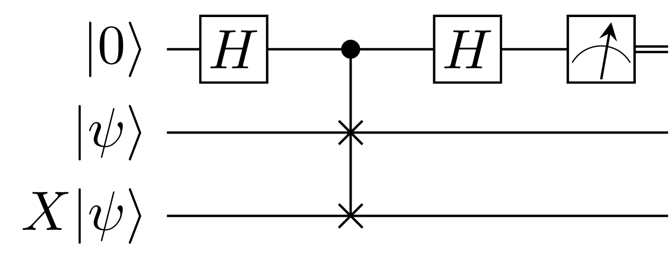
Let’s try to obtain the same result using Monte Carlo integration. This is important because it allows us to validate the basic scheme used to compute $\lvert \bra{\psi}X\ket{\psi} \rvert^2$. This scheme is just the SWAP test.

Average of a function over the Bloch sphere: Monte Carlo integration

The procedure to compute the average is very similar to Equation $(9)$ except now we need to generate Haar-random states:

Where $\ket{\psi}$ is chosen randomly according to the Haar measure.

In our specific case, the function is given by Equation $(12)$ so Equation $(14)$ reads:

As we’ve repeatedly alluded to, $\lvert \bra{\psi} X \ket{\psi} \rvert^2$ is calculated using the SWAP test which can be seen in the figure below:

SWAP test: our goal is to compare how much the states $\ket{\psi}$ and $X\ket{\psi}$ are similar, outputing how probable the two states are similar.

Back to the business of generating Haar-random states, we need to generate a random unitary matrix in $U(2)$ and using it we can generate a Haar-random state. (Ozols, 2009) in section $2.3$ shows a method to generate a random matrix from $U(2)$ but we won’t use that method because it is not our goal to learn how to generate either random states or random matrices.
Instead, we will use Scipy to do the heavy lifting for us: it is as simple as importing unitary_group from scipy.stats then specifying the dimension of the unitary we wish to get, in our case $2$.

The code below computes the average fidelity as we wish:

import pennylane as qml

from scipy.stats import unitary_group as ug

def swap_test(state_prep_unitary):
    n_shots = 50_000
    dev = qml.device(
        "default.qubit",
        wires = 3,
        shots = n_shots
    )

    @qml.qnode(dev)
    def swap_test_circuit():
        # Prepare the state |psi> on qubit 1
        qml.QubitUnitary(state_prep_unitary, wires = 1)

        # Prepare the state X|psi> on qubit 2
        qml.QubitUnitary(state_prep_unitary, wires = 2)
        qml.PauliX(wires = 2)

        # Perform the SWAP test
        qml.Hadamard(wires = 0)
        qml.CSWAP(wires = [0, 1, 2])
        qml.Hadamard(wires = 0)

        # Collect counts on qubit 0
        return qml.counts(qml.PauliZ(0))

    dist = swap_test_circuit()
    one_state_count = dist[-1] if -1 in dist else 0
    return 1 - (2 / n_shots) * one_state_count

def monte_carlo_average(f, sample_size):
    total = 0

    for _ in range(sample_size):
        # ug.rvs will sample a random nxn matrix from the unitary group
        total += f(ug.rvs(2))

    return total / sample_size

if __name__ == "__main__":
    print(monte_carlo_average(swap_test, 5_000))

Notice also that we make $25\times 10^7$ calls to the quantum “computer” which is a large number of calls. Using states designs, we will reduce that to $3\times 10^4$ which is more than an $800$-fold decrease in the number of calls.

Average of a function over the Bloch sphere: state designs

Computing the average of a function of a quantum state is akin to computing the average over spheres. The only difference now is that we are supposed to choose specific states, and in the case of single-qubit states, we need to choose states on the Bloch sphere.

First, we define state designs:

Definition: let $f_t$ be a polynomial in $t$ variables homogeneous in degree at most $t$ in those variables and degree $t$ in the complex conjugate of those variables. A set $X = \{ \ket{\psi} \vert \ket{\psi} \in \mathcal{S}(\mathbb{C}^{2^n}) \}$ is a state $t$-design if:

\[\dfrac{1}{\lvert X \rvert} \sum_{\ket{\psi} \in X} f_t(\ket{\psi}) = \dfrac{1}{Vol(\mathcal{S}(\mathbb{C}^{2^n}))} \int_{\mathcal{S}(\mathbb{C}^{2^n})} f_t(\ket{\psi}) d_{\mu}\ket{\psi} \tag{15}\]

holds for all possible $f_t$. Moreover a quantum state $t$-design is also a quantum state $s$-design for all $0 < s < t$.

The definition is pretty familiar at this point but one aspect deserves a comment: $f_t$ is a polynomial in $t$ variables homogeneous in degree at most $t$ in those variables and degree $t$ in the complex conjugate of those variables.

What that means is that we should have an equal number of kets $\ket{\psi}$ and an equal number of bras $\bra{\psi}$ in the function $f_t$.
In the case of $f_2(\ket{\psi}) = \bra{\psi}\mathcal{E}(\ket{\psi}\bra{\psi})\ket{\psi}$ we have exactly two $\ket{\psi}$ and two $\bra{\psi}$, so our function is homogeneous in degree $2$.

((Kaznatcheev, 2009) has more examples and details, the reader is encouraged to read it.)

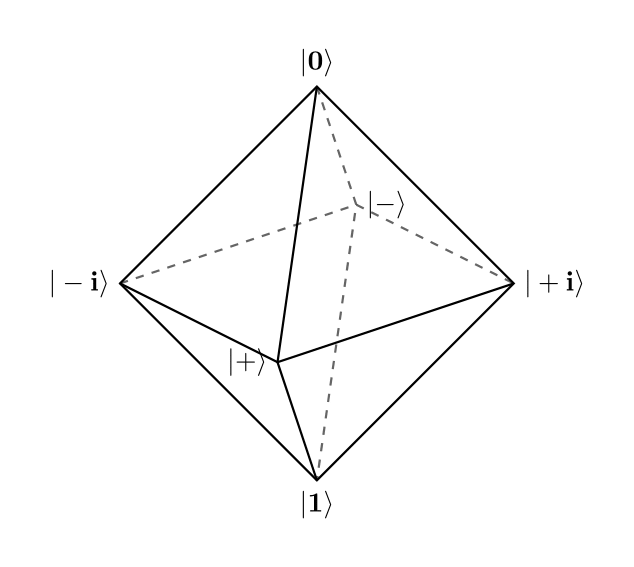
It can be shown that the eigenvectors of Pauli matrices, $P = \{\ket{0}, \ket{1}, \ket{+}, \ket{-}, \ket{+i}, \ket{-i}\}$, form a state $3$-design (and therefore a $2$-design) since when connected they form an octahedron as in the figure below:

Pauli states are a $3$-design: when plotted inside the Bloch sphere and connected by lines, the eigenvectors of Pauli matrices form an octahedron.

Let’s try to calculate the average fidelity of $X$ using our state $2$-design.

Since our function is relatively simple and we only have $6$ states, we can easily analytically compute the average using Equation $(15)$ then do the same computation again in software:

Which is in excellent agreement with the results we got thus far. We now code that up to finalize:

import numpy as np
import pennylane as qml

def zero(wire):
    # This non-circuit prepares the |0> state
    pass

def one(wire):
    # This circuit prepares the |1> state
    qml.PauliX(wires = wire)

def plus(wire):
    # This circuit prepares the |+> state
    qml.Hadamard(wires = wire)

def minus(wire):
    # This circuit prepares the |-> state
    qml.PauliX(wires = wire)
    qml.Hadamard(wires = wire)

def plus_i(wire):
    # This circuit prepares the |+i> state
    qml.Hadamard(wires = wire)
    qml.S(wires = wire)

def minus_i(wire):
    # This circuit prepares the |-i> state
    qml.PauliX(wires = wire)
    qml.Hadamard(wires = wire)
    qml.S(wires = wire)

def swap_test(state_prep_gate):
    n_shots = 50_000
    dev = qml.device(
        "default.qubit",
        wires = 3,
        shots = n_shots
    )

    @qml.qnode(dev)
    def swap_test_circuit():
        # Prepare the state |psi> on qubit 1
        state_prep_gate(1)
        
        # Prepare the state X|psi> on qubit 2
        state_prep_gate(2)
        qml.PauliX(wires = 2)

        # Perform the SWAP test
        qml.Hadamard(wires = 0)
        qml.CSWAP(wires = [0, 1, 2])
        qml.Hadamard(wires = 0)

        # Collect counts on qubit 0
        return qml.counts(qml.PauliZ(0))

    dist = swap_test_circuit()
    one_state_count = dist[-1] if -1 in dist else 0
    return 1 - (2 / n_shots) * one_state_count

def state_design_average(f, states):
    return np.mean([f(state) for state in states])

if __name__ == "__main__":
    print(state_design_average(
        swap_test,
        [zero, one, plus, minus, plus_i, minus_i]
    ))

And thus, using state designs, we have managed to calculate the average fidelity of the $X$ gate using $3\times 10^4$ samples, instead of the $25\times 10^7$ that we used for Monte Carlo integration. That’s going from $250$ millions to $30$ thousand, a huge reduction in the number of samples.

Not only that, finding the average analytically using sums over the $2$-design set (Pauli eigenvectors) was simpler than doing integration!

It is therefore to our advantage to use designs than other methods whenever the situtation lends itself to their use.

In the coming subsection, we are going to find the average fidelity of the Pauli $X$ gate subject to calibration noise using state designs.

Application: average gate fidelity

Assume that the only noise the Pauli $X$ gate is subject to is a stochastic calibration noise.

The $X$ gate is a rotation about the x-axis by $\pi$ radians up to an irrelevant global phase:

Let’s say that our implementation is not perfect and instead of having $X = RX(\pi)$ we end up with $X_{\epsilon} = RX(\pi + \hat{\epsilon})$ where $\hat{\epsilon}$ is a random variable with zero-mean and standard deviation $\sigma$.

Our goal is to calculate the average fidelity of the implemented gate $X_{\epsilon}$ with respect to the ideal gate $X$.
In general, we should expect that in case on no calibration error, that is $\hat{\epsilon}$ has zero-mean and zero standard deviation, $X_{\epsilon} = X$. And we also expect that as we increase the standard deviation, we will get farther away from the ideal $X$ gate.

Let us formulate the problem in a general way: let $G$ be the ideal gate and $G_{\epsilon}$ be the gate subject to some sort of error. There is no requirement that the error be a calibration error, it can be any other such as incoherent errors.

We wish to calculate the average fidelity of the gate $G_{\epsilon}$ with respect to the ideal gate $G$. (To simplify the language, we will simply say that we wish to find the average fidelity of $G_{\epsilon}$.)

To do the same, we need to find how probable the states $G_{\epsilon} \ket{\psi}$ are the same as the states $G \ket{\psi}$.

The average fidelity is given by:

In our case where we are dealing with single-qubit gates $X_{\epsilon}$ and $X$, Equation $(16)$ specializes to:

Immediately, we can see that it is no fun trying to calculate that integral by hand. This is especially true if we had more complex noise channels describing $X_{\epsilon}$. Even more so on real devices where gates are subject to much more complicated noise channels.

Fornunately we have designs to our rescue: we will use the exact procedure as above with the difference now being that we need to incorporate the action of $X_{\epsilon}$ on the state $\ket{\psi}$ chosen from eigenvectors of Pauli matrices:

Average gate fidelity of $X_\epsilon$: we compare how probable the state created by $X_\epsilon$ is equal to the state create by $X$.

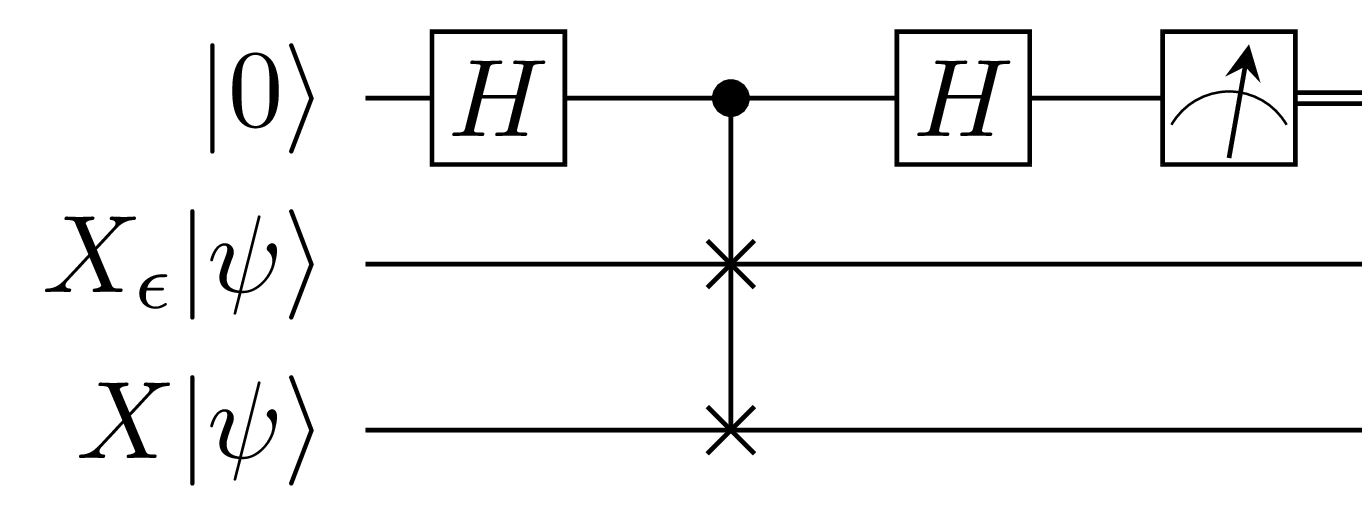
The code that follows computes the average gate fidelity as per the circuit above:

import numpy as np
import pennylane as qml


def zero(wire):
    # This non-circuit prepares the |0> state
    pass

def one(wire):
    # This circuit prepares the |1> state
    qml.PauliX(wires = wire)

def plus(wire):
    # This circuit prepares the |+> state
    qml.Hadamard(wires = wire)

def minus(wire):
    # This circuit prepares the |-> state
    qml.PauliX(wires = wire)
    qml.Hadamard(wires = wire)

def plus_i(wire):
    # This circuit prepares the |+i> state
    qml.Hadamard(wires = wire)
    qml.S(wires = wire)

def minus_i(wire):
    # This circuit prepares the |-i> state
    qml.PauliX(wires = wire)
    qml.Hadamard(wires = wire)
    qml.S(wires = wire)

def PauliX_e(angle, wire):
    qml.RX(np.pi + angle, wires = wire)

def swap_test(state_prep_gate, calibration_error_angle):
    n_shots = 50_000
    dev = qml.device(
        "default.qubit",
        wires = 3,
        shots = n_shots
    )

    @qml.qnode(dev)
    def swap_test_circuit():
        # Prepare the state X\_e|psi> on qubit 1
        state_prep_gate(1)
        PauliX_e(calibration_error_angle, 1)
        
        # Prepare the state X|psi> on qubit 2
        state_prep_gate(2)
        qml.PauliX(wires = 2)

        # Perform the SWAP test
        qml.Hadamard(wires = 0)
        qml.CSWAP(wires = [0, 1, 2])
        qml.Hadamard(wires = 0)

        return qml.counts(qml.PauliZ(0))

    dist = swap_test_circuit()
    one_state_count = dist[-1] if -1 in dist else 0
    return 1 - (2 / n_shots) * one_state_count

def state_design_average(f, calibration_error_angle, states):
    return np.mean([f(state, calibration_error_angle) for state in states])

if __name__ == "__main__":
    """
    Ideally the calibration error angles will be random.
    We use deterministic angles of increasing value to demonstrate
    that the average fidelity decreases as the error angle increases.
    """
    calibration_error_angles = [0, np.pi/2, np.pi]
    for calibration_error_angle in calibration_error_angles:
        print(f"Fidelity at angle error {calibration_error_angle} =",
            state_design_average(
                swap_test,
                calibration_error_angle,
                [zero, one, plus, minus, plus_i, minus_i]
            )
        )

Here are the results of my run locally:

Fidelity at angle error 0 = 1.0
Fidelity at angle error 1.5707963267948966 = 0.6677266666666667
Fidelity at angle error 3.141592653589793 = 0.33261333333333326

And there it is: we were able to calculate by how much a gate subject to some error is different from the ideal gate.

In the next section, we introduce unitary designs then use them to do the same computation of the average gate fidelity.

Unitary designs

In the previous section, we were able to average a function over quantum states by randomly sampling said states.
But note that in order to generate those random states, we actually randomly sampled unitaries then applied the random unitary to a fudiciary starting state.

Sure, we could have randomly sampled from $\mathcal{S}(\mathbb{C}^{2^n})$ then synthesize a circuit that prepares that state but we would have been bothering ourselves solving a problem useless to our mission of understand designs.

Therefore it stands to reason that it makes more sense to have functions that depend not on states but on unitaries. Moreover unitaries are nicer than states: they form a group so we can combine them under the group operation if we need to.

In this section we look at functions that depend on unitaries and not quantum states and how to average such functions. As application, we will again calculate the average fidelity of the Pauli $X$ gate but now by averaging over unitaries.

Functions of a unitary and their average

A function of a unitary is a function that takes a unitary matrix as input and can output some other quantity depending on the form of the function.
In general the codomain of the function doesn’t matter for the math so long as we can interpret the output we get.

Otherwise the form of such a function is similar to functions we have seen thus far, the only difference now is that these functions take unitary matrices as input.

Functions of a unitary

Let $U$ be a unitary from $U(2^n) \subset \mathbb{C}^{2^n} \times \mathbb{C}^{2^n}$, the set of unitary matrices acting on $n$ qubits. We are interested in functions that take unitaries such as $U$ as input.

Functions over unitaries can have a variety of codomains:

• $U(2^n)$: a function that corresponds to the commutator between $U, V \in U(2^n)$ will output a matrix in $U(2^n)$.
• $\mathbb{C}^{2^n}$: a function corresponding to the application of a unitary to a quantum state $\ket{\psi} \in \mathbb{C}^{2^n}$ will output a quantum state in $\mathbb{C}^{2^n}$.
• $\mathbb{R}$: a function that computes the distance between two quantum states such as $\lvert\bra{\psi}U\ket{\psi}\rvert^2$ will output a real number.

And so on. So we can’t readily define the codomain of functions over unitaries until we are precise about what are computing.

Nonetheless, to get our feet in the waters, we will start with two functions that correspond to the conjugation of a square matrix $M$ by a unitary.

The single-qubit case is given by:

And the two-qubits case is given by:

Where $U, U_A, U_B \in U(2)$ and $M$ are square matrices of dimensions $2^n \times 2^n$. Even this dimension is a hard requirement that need not be but we impose it because all the matrices we will be working with will be either quantum gates or density matrices.

Both functions will help us introduce averaging over functions of unitaries, and think about what the obtained results mean.

Then in the application subsection we will rephase the calculation of the average gate fidelity given by Equation $(16)$ as an integral over unitaries instead of quantum states.

Average of a function of unitaries

The average of a function of unitaries is similar to that of a function of quantum states. The only difference is that we need to be careful about the calculation of the volume element, as usual.

Similar to Equation $(13)$, the average of a function of unitaries is given by:

Where the volume element is calculated with respect to the Haar measure. The calculation of this volume element is not necessarily trivial for arbitrary system sizes as can be seen in (Tilma & Sudarshan, 2004) who have carried out these calculations.

On the plus side, since our goal is to understand enough to write software that calculates the average, and not necessarily carry out the calculations by hand, it will suffice to use precalculated results.

In fact, for our two functions of interest, it is not even necessary to find the volume element $d_{\mu}U$: integration over the Haar measure mostly amounts to using properties of the Haar measure.
And even in that case our goal is not to learn how to evaluate integrals over the unitary group. The integrals we will care about in this post have been evaluated in (Zhang, 2015). We will simply reuse the results therein.

Average of a function of a unitary: analytic solution

We present the analytic solutions of the average of the two functions of interest and we interpret the obtained result when the conjugated matrix $M$ is a density matrix.

Before we start, recall that we said that sometimes it is assumed that the Haar measure is uniform. That simply means that we don’t need to divide by the volume and simply take it that the Haar measure is uniform. In this case the average is simplified and is given by:

Where the volume element $dU$ has the Haar measure already divided by the volume (it is uniform). The calculations that lead to the relevant solutions assume this to be the case.

Function in one variable

(See subsection $3.1$, Equation $(3.6)$ in (Zhang, 2015).)

In the first case, for the function where the unitary we are integrating over act on single qubit, the average is given by:

Where $\mathbb{1}$ is the identity matrix on $1$ qubit.

We recognize $\frac{\text{Tr}[M]}{2} \mathbb{1}$ as the completely mixed state if $M$ is a density matrix. The interpretation of the result obtained is that the averaging procedure transforms any density matrix into the completely mixed state. Therefore the averaging procedure acts as the fully depolarizing channel.

This is easily realized by remembering that a valid density matrix must have unit trace therefore Equation $(18)$ will result in $\frac{1}{2} \mathbb{1}$ which is the completely mixed state for a single qubit.

It is worth recalling that $M$ doesn’t need to be a density matrix, it can any square matrix. Even though we may use them for testing, it is not obvious how to interpret the result.

For instance, consider $M = X$ where $X$ is the Pauli $X$ matrix. Averaging over it, we obtain:

While the null matrix is indeed a unitary matrix, it is not a valid quantum gate so we can’t say that overaging over the Pauli $X$ results in a particular quantum gate.

It follows that in the general case, we shouldn’t draw a conclusion of the kind: averaging over a quantum gate results in another quantum gate.

Function in two variables

(See subsection $3.1$, Equation $(3.10)$ in (Zhang, 2015).)

In the second case, for the function where the unitaries we are integrating over act separately acting on two qubits, the average is given by:

Where $\mathbb{1}_A$ is the identity matrix on the first qubit, and $\mathbb{1}_B$ is the indentity matrix on the second qubit.

Equation $(19)$ is the fully depolarizing channel for two qubits.

Average of a function of a unitary: Monte Carlo integration

Recalling that every density matrix has unit trace, it is not interesting to compute Equations $(18)$ and $(19)$ using Monte Carlo integration.

Instead, for the single-qubit and two qubits integrals, we will use some quantum gates so as to convince ourselves that Monte Carlo integration recovers the expected analytical result.

Function in one variable

The Monte Carlo integration for the single-qubit integral is given by:

For instance, for $S = \begin{bmatrix} 1 & 0 \\ 0 & i \end{bmatrix}$ (the phase gate), the average of $f(U) = U S U^\dagger$ is given by:

Using Monte Carlo integration, we obtain the same result. The code follows performs the same calculation as above:

import numpy as np

from scipy.stats import unitary_group as ug

# Limit the number of decimal digits to 2
np.set_printoptions(precision = 2, suppress = True)

def monte_carlo_average(M, n_samples):
    R = np.zeros(M.shape)
    for _ in range(n_samples):
        U = ug.rvs(2)
        R = R + (U @ M @ U.conj().T)
    return (1 / n_samples) * R

if __name__ == "__main__":
    S = np.matrix([
        [1, 0],
        [0, 1j]
    ])
    print(monte_carlo_average(S, 50_000))

Function in two variables

The Monte Carlo integration for the two qubits integral is given by:

As an example, take $CNOT = \begin{bmatrix} 1 & 0 & 0 & 0 \\ 0 & 1 & 0 & 0 \\ 0 & 0 & 0 & 1 \\ 0 & 0 & 1 & 0 \end{bmatrix}$, the average of $f(U_A, U_B) = (U_A \otimes U_B) \, CNOT \, (U_A \otimes U_B)^\dagger$ is given by:

The average using Monte Carlo integration is computed by the code that follows:

import numpy as np

from scipy.stats import unitary_group as ug

# Limit the number of decimal digits to 2
np.set_printoptions(precision = 2, suppress = True)

def monte_carlo_average(M, n_samples):
    R = np.zeros(M.shape)
    for _ in range(n_samples):
        U_i = ug.rvs(2)
        for _ in range(n_samples):
            U_j = ug.rvs(2)
            R = R + (np.kron(U_i, U_j) @ M @ np.kron(U_i, U_j).conj().T)
    return (1 / n_samples**2) * R

if __name__ == "__main__":
    CNOT = np.matrix([
        [1, 0, 0, 0],
        [0, 1, 0, 0],
        [0, 0, 0, 1],
        [0, 0, 1, 0],
    ])
    # We know the resulting matrix is real
    # so we make sure to take only the real parts of each entry
    print(monte_carlo_average(CNOT, 2_000).real)

Average of a function of a unitary: unitary designs

Having computing the integrals using Monte Carlo integration, it is time to compute the same using unitary designs.

Let’s begin by defining what a unitary $t$-designs are then we will show how to check whether a set is a $1$-design or a $2$-design.

Definition: let $f_t$ be a polynomial in $t$ variables homogeneous in degree at most $t$ in those variables and degree $t$ in the Hermitian transpose of those variables. A set $X = \{ U \vert U \in U(2^n) \}$ is a unitary $t$-design if:

\[\dfrac{1}{\lvert X \rvert} \sum_{U \in X} f_t(U) = \int_{U({2^n})} f_t(U) dU \tag{22}\]

holds for all possible $f_t$, with $dU$ being the volume element with uniform Haar measure. Moreover a unitary $t$-design is also a unitary $s$-design for all $0 < s < t$.

The definition is pretty similar to that of state designs but now we require that each term in the function $f_t$ contains an equal number of unitaries and their Hermitian transposes.

For instance $f_t(U_A, U_B) = U_A^\dagger U_B^\dagger U_A U_B$ will pass since it has two unitaries and two Hermitian transposes of those unitaries.

On the other hand $f_t(U_A, U_B) = U_A U_B U_A^\dagger$ will not pass even though it is homogeneous: it has an unequal number unitaries ($2$) and their complex conjugates ($1$).

For our functions of interest, $f = UMU^\dagger$ has one unitary and one Hermitian transpose of that unitary so it is a polynomial that’s homogeneous of degree $1$. We will therefore require a $1$-design to compute it.

The function $f = (U_A \otimes U_B)M_{AB}(U_A \otimes U_B)^\dagger$ has two unitaries and two Hermitian transposes of those unitaries so it is a polynomial of degree $2$. We will need a $2$-design to compute it.

Unitary 1-design

Having defined what unitary $t$-designs are, how do we check if a particular set is a $1$-design?

A set $X$ is a unitary $1$-design if and only if (Roy & Scott, 2009):

Where $P_{ji}$ is a permutation that maps the basis elements $\ket{ij}$ to $\ket{ji}$, (effectively the two-qubits SWAP gate). If we are dealing with $4$ qubits, $P_{21}$ will map $\ket{ijkl}$ to $\ket{klij}$.

The proof that $\int_{U({2^n})} U \otimes U^\dagger dU = \dfrac{P_{21}}{2^n}$ can be found in Subsection $3.1$, Corollary $3.5$ of (Zhang, 2015).

It is the case that the Pauli group is a $1$-design. We now verify using Equation $(23)$. Please make sure to have the supplementary materials code where we generate the Pauli group and the permutation matrix $P_{21}$.

import numpy as np
import itertools as it

from typing import List, Tuple

class Permutation:
    # Please copy and paste the code from the supplementary material here
    pass

class Pauli:
    # Please copy and paste the code from the supplementary material here
    pass

def is_unitary_1_design(group):
    R = np.asmatrix(np.zeros((4,4)))

    for element in group:
        R = R + np.kron(element, element.H)
    
    F = (1 / len(group)) * R
    P_21 = Permutation(2).get_permutation_matrix([2, 1])
    return np.allclose(F, P_21 / 2)

if __name__ == "__main__":
    print(is_unitary_1_design(Pauli.group()))

Now that we have validated that the Pauli group is a $1$-design, we can proceed to use to compute the average of our function of interest $f = U\,M\,U^\dagger$.

The procedure is exactly the same as computing the average using Monte Carlo integration except instead of sampling $U$ randomly, we take it from the Pauli group:

The code that computes the average using the Pauli group is:

import numpy as np

class Pauli:
    # Please copy and paste the code from the supplementary material here
    pass

def unitary_design_average(M, t_design):
    R = np.zeros(M.shape)
    for U in t_design:
        R = R + (U @ M @ U.conj().T)
    return (1 / len(t_design)) * R

if __name__ == "__main__":
    S = np.matrix([
        [1,  0],
        [0, 1j]
    ])
    print(unitary_design_average(S, Pauli.group()))

In computing this average using Monte Carlo integration, we used about $50,000$ samples in order to account for the way statistics work: the more samples we use, the better will our results be.

With designs, in this case the Pauli group, we used $4$ elements only and we got our result which is also exact! With Monte Carlo, I suppose we could use $40$ samples but we can see how quickly we will loose accuracy and we still wouldn’t beat the loop that run just $4$ times.

Unitary 2-design

Equivalently, a set $X$ is a unitary $2$-design if and only if (Roy & Scott, 2009):

Where $P_{lkji}$ is a permutation that maps the basis elements $\ket{ijkl}$ to $\ket{lkji}$.

The proof that $\int_{U({2^n})} U^{\otimes 2} \otimes (U^\dagger)^{\otimes 2} \, dU = \dfrac{P_{3412} + P_{4321}}{4^n - 1} - \dfrac{P_{4312} + P_{3421}}{2^n(4^n - 1)}$ can be found in Subsection $3.2$, Corollary $3.15$ of (Zhang, 2015).

Our $2$-design set is the Clifford group (Matteo, 2014). We can verify this by using Equation $(24)$, same as we did for the Pauli group. Note also that since the Clifford group is a $2$-design, it is also a $1$-design. In fact, the Clifford group has been proven to be a $3$-design (Webb, 2016) but since we are not using anything that requires $3$-designs, we won’t delve into that. On the other hand, the Pauli group is uniquely a $1$-design.

import numpy as np
import itertools as it
import scipy.linalg as la

from collections import deque
from typing import List, Tuple

class Permutation:
    # Please copy and paste the code from the supplementary material here
    pass

def matrix_in_list(element, list):
    # Please copy and paste the code from the supplementary material here
    pass

def matrix_is_normalizer(x):
    # Please copy and paste the code from the supplementary material here
    pass

class Pauli:
    # Please copy and paste the code from the supplementary material here
    pass

class Clifford:
    # Please copy and paste the code from the supplementary material here
    pass

def is_unitary_1_design(group):
    R = np.asmatrix(np.zeros((4,4)))

    for element in group:
        R = R + np.kron(element, element.H)
    
    F = (1 / len(group)) * R
    P_21 = Permutation(2).get_permutation_matrix([2, 1])

    return np.allclose(F, P_21 / 2)

def is_unitary_2_design(group):
    R = np.asmatrix(np.zeros((16,16)))
    for element in group:
        element_d = element.H
        R = R + np.kron(
            np.kron(element, element),
            np.kron(element_d, element_d)
        )

    F = (1 / len(group)) * R
    P_3412 = Permutation(4).get_permutation_matrix([3, 4, 1, 2])
    P_3421 = Permutation(4).get_permutation_matrix([3, 4, 2, 1])
    P_4321 = Permutation(4).get_permutation_matrix([4, 3, 2, 1])
    P_4312 = Permutation(4).get_permutation_matrix([4, 3, 1, 2])

    return np.allclose(
        F,
        (P_3412 + P_4321) / 3 - (P_4312 + P_3421) / 6
    )

if __name__ == "__main__":
    print("Clifford group is 2-design:",
        is_unitary_2_design(Clifford.group()))
    print("Clifford group is 1-design:",
        is_unitary_1_design(Clifford.group()))

    print("Pauli group is 2-design:",
        is_unitary_2_design(Pauli.group()))
    print("Pauli group is 1-design:",
        is_unitary_1_design(Pauli.group()))

Our second function of interest is a polynomial homogeneous in degree $2$ so computing its average requires a $2$-design which we now have.

Computing the average of $f = (U_A \otimes U_B) M_{AB} (U_A \otimes U_B)^\dagger$ is exactly the same procedure as we did for Monte Carlo integration except instead of sampling randomly, we use the Clifford group elements.

import numpy as np
import scipy.linalg as la

from collections import deque

# Limit the number of decimal digits to 2
np.set_printoptions(precision = 2, suppress = True)

def matrix_in_list(element, list):
    # Please copy and paste the code from the supplementary material here
    pass

def matrix_is_normalizer(x):
    # Please copy and paste the code from the supplementary material here
    pass

class Pauli:
    # Please copy and paste the code from the supplementary material here
    pass

class Clifford:
    # Please copy and paste the code from the supplementary material here
    pass

def unitary_design_average(M, t_design):
    R = np.zeros(M.shape)
    for U_i in t_design:
        for U_j in t_design:
            R = R + (np.kron(U_i, U_j) @ M @ np.kron(U_i, U_j).conj().T)
    return (1 / len(t_design)**2) * R

if __name__ == "__main__":
    CNOT = np.matrix([
        [1, 0, 0, 0],
        [0, 1, 0, 0],
        [0, 0, 0, 1],
        [0, 0, 1, 0],
    ])
    # We know the resulting matrix is real
    # so we make sure to take only the real parts of each entry
    print(unitary_design_average(CNOT, Clifford.group()).real)

Compared to the $2\times 10^6$ iterations we used for Monte Carlo integration, $576$ iterations using unitary designs is a real bargain.

Application: average gate fidelity

We were able to calculate the average gate fidelity using state designs. We compute the same now using unitary designs.

We begin by reformulating the problem in terms of integration over the unitary group instead of states.

Let’s recall the formula for calculating the average gate fidelity of $G_\epsilon$ given the ideal gate $G$:

To simplify our reasoning process, let’s first assume that the Haar measure is uniform, that is $d\ket{\psi} = \frac{d_{\mu}\ket{\psi}}{Vol(\mathcal{S}(\mathbb{C}^{2^n}))}$:

Instead of creating random states $\ket{\psi}$ by randomly generating unitaries $U$ such as $\ket{\psi} = U\ket{0}$, we generate said unitaries $U$ randomly and integrate over the unitary group:

We can see that our function of interest $f = \bra{0}U^\dagger G^{\dagger} \cdot G_{\epsilon}(U\ket{0}\bra{0}U^\dagger) \cdot G U\ket{0}$ has two unitaries $U$ and two Hermitian transposes of the same unitary. It follows that averaging this function over the unitary group requires a $2$-design. We will of course make use of the Clifford group.

Our goal is to perform the computation:

Where we have set $G_\epsilon = X_\epsilon$ and $G = X$, $X$ is the Pauli $X$ gate and $X_\epsilon$ is the $X$ gate subject to coherent noise.

Each $U$ is taken from the Clifford group $\mathcal{C}$. The code remains essentially the same as that for computing the average fidelity using state designs but instead of passing states to the SWAP test, we pass unitaries from the Clifford group.

import numpy as np
import pennylane as qml
import scipy.linalg as la

from collections import deque


def matrix_in_list(element, list):
    # Please copy and paste the code from the supplementary material here
    pass

def matrix_is_normalizer(x):
    # Please copy and paste the code from the supplementary material here
    pass

class Pauli:
    # Please copy and paste the code from the supplementary material here
    pass

class Clifford:
    # Please copy and paste the code from the supplementary material here
    pass

def PauliX_e(angle, wire):
    # We add a randomly generated angle to simulate
    # stochastic calibration noise
    qml.RX(np.pi + angle, wires = wire)

def swap_test(state_prep_unitary, calibration_error_angle):
    n_shots = 50_000
    dev = qml.device(
        "default.qubit",
        wires = 3,
        shots = n_shots
    )

    @qml.qnode(dev)
    def swap_test_circuit():
        # Prepare the state X\_e|psi> on qubit 1
        qml.QubitUnitary(state_prep_unitary, wires = 1)
        PauliX_e(calibration_error_angle, 1)

        # Prepare the state X|psi> on qubit 2
        qml.QubitUnitary(state_prep_unitary, wires = 2)
        qml.PauliX(wires = 2)

        # Perform the SWAP test
        qml.Hadamard(wires = 0)
        qml.CSWAP(wires = [0, 1, 2])
        qml.Hadamard(wires = 0)

        # Collect counts on qubit 0
        return qml.counts(qml.PauliZ(0))

    dist = swap_test_circuit()
    one_state_count = dist[-1] if -1 in dist else 0
    return 1 - (2 / n_shots) * one_state_count

def unitary_design_average(f, calibration_error_angle, unitaries):
    return np.mean([f(unitary, calibration_error_angle) for unitary in unitaries])

if __name__ == "__main__":
    """
    Ideally the calibration error angles will be random.
    We use deterministic angles of increasing value to demonstrate
    that the average fidelity decreases as the error angle increases.
    """
    calibration_error_angles = [0, np.pi/2, np.pi]
    group = Clifford.group()
    for calibration_error_angle in calibration_error_angles:
        print(f"Fidelity at angle error {calibration_error_angle} =",
            unitary_design_average(
                swap_test,
                calibration_error_angle,
                group
            )
        )

We have confirmed that we can calculate the average fidelity using unitary designs instead of state designs.

If were dealing with a two qubits gate, we could use the Clifford on two qubits (by adding the $CNOT$ gate to the generating set), and that would be easier than using state designs.

Next steps

As quantum software developers/engineers, we need to get acquainted with the mathematics and physics behind the numerous techniques discovered by scientists so we can choose the best tool for the job at hand.

Initially, we need to learn the minimum mathematics and physics required to use the technique (write software). This blog post was all about learning that minimum so that we can appreciate the technique.

Eventually the need may arise where we need to actually learn the mathematics and physics deeper so we can follow along more sophisticated papers and/or help scientists we are working with.

Towards that goal, here are some resources to hit that road:

• Antonio Anna Mele has a nice article that covers the mathematics related to the Haar measure in (Mele, 2024).
• Lin Zhang’s article (Zhang, 2015) with detailed calculations is a good starting point to learn how to do such calculations by hand.
• Olivia Di Matteo’s article (Matteo, 2014) has a detailed derivation of the fact that the Clifford group is a $2$-design. This is good to help practice such calculations using a guide. Moreover, their tutorials on unitary designs and Haar measure are great. For instance, we never elaborated how to generate random unitaries, this is covered in their tutorial on the Haar measure. Moreover, their method of finding the average fidelity is worth experimenting with instead of using the SWAP test as we did in this article (it is the method to use if some state tomography was done).

After getting better acquainted with the basic mathematics behind unitary designs, it is worth exploring the different facets of quantum designs in general such as approximate designs, the concept of frame, etc, and their applications.

Conclusion

In this tutorial, we have learned the basics of quantum designs, namely state designs and unitary designs and used them to solve a practical problem: finding the average fidelity of a quantum gate.

Quantum designs are but another tool we use to solve some of the many challenging problems we encounter in quantum computing; in our instance to get around the cost of gate (set|process) tomography.

The reader is encouraged to explore other areas where they are used, and an instance is finding the expressibility of a quantum circuit as needed in variational quantum circuits by following (Sim et al., 2019).

Supplementary material

There were procedures we needed to carry out that were important to understand the material but it made no sense to have in the main text.

The supplements that follow contain code to help carry out those procedures without cluttering the main text.

Generating permutation matrices

In the subsection on computing the average of a function of unitaries using unitary designs, we need to generate permutation matrices so we can check whether a given set is a $1$-design or a $2$-design. This supplement is about how to do that.

A permutation matrix simply exchanges basis elements. For instance, the permutation $P_{21}$ has the effect of of swapping basis elements such that if the basis element is $\ket{ij}$ then $P_{21}\ket{ij} = \ket{ji}$. The result will be as follows:

On the other hand the permutation $P_{3412}$ has the effect of swapping basis elements such as $P_{3412}\ket{i_1j_2k_3l_4} = \ket{k_3l_4i_1j_2}$. The result will be as follows:

As we can see, we are just exchanging values at the given indices. Our goal is to generate the matrices that correspond to those permutations.

We adopt a 3-steps plan:

1. Generate the basis elements corresponding to the number of qubits.
2. Generate a list where each item is a tuple that tells which basis element maps to which basis element.
3. Generate the permutation matrix based on the list generated above.

Step $1$ is fairly trivial: say we have $n$ qubits. If $n = 1$ then we are done: $\mathcal{B}_1 = \{\ket{0}, \ket{1} \}$. If $n = 2$ then the basis set is the Cartesian product of two single-qubit basis sets: $\mathcal{B}_2 = \mathcal{B}_1 \times \mathcal{B}_1$. If $n = 3$ then the basis set is the Cartesian product of a two-qubits basis set and a single-qubit basis set: $\mathcal{B}_3 = \mathcal{B}_2 \times \mathcal{B}_1$.

In general, for $n > 1$ qubits we have:

Let’s readily code the same:

import itertools as it
import numpy as np

class Permutation:
    def __init__(self, n_qubits: int):
        if n_qubits < 1:
            raise ValueError("The number of qubits must be at least 1")
        self.n_qubits = n_qubits
    
    def get_basis_set(self):
        single_qubit_basis = ['0', '1']
        new_basis = single_qubit_basis
        temp_basis = []
        for _ in range(self.n_qubits - 1):
            for r in it.product(new_basis, single_qubit_basis):
                temp_basis.append(r[0] + r[1])
            new_basis = temp_basis
            temp_basis = []
        return new_basis
    
if __name__ == "__main__":
    permutation = Permutation(2)
    print(permutation.get_basis_set())

Moving onto step $2$: as we have already seen, the procedure is to take every basis element and make the appropriate replacement as dictated by the permutation formula. For example, assume again that the replacement formula is given by $P_{3412}\ket{i_1j_2k_3l_4} = \ket{k_3l_4i_1j_2}$. To generate the new basis element, starting from $\ket{\psi} = \ket{i_1j_2k_3l_4}$, we perform the replacements $\ket{\psi}[1] = k_3$, $\ket{\psi}[2] = l_4$, $\ket{\psi}[3] = i_1$, and $\ket{\psi}[4] = j_2$.
Of course since we are writing Python, we remain mindful of indices starting at $0$.

import itertools as it
import numpy as np

from typing import List, Tuple

class Permutation:
    def __init__(self, n_qubits: int):
        if n_qubits < 1:
            raise ValueError("The number of qubits must be at least 1")
        self.n_qubits = n_qubits
    
    def get_basis_set(self):
        single_qubit_basis = ['0', '1']
        new_basis = single_qubit_basis
        temp_basis = []
        for _ in range(self.n_qubits - 1):
            for r in it.product(new_basis, single_qubit_basis):
                temp_basis.append(r[0] + r[1])
            new_basis = temp_basis
            temp_basis = []
        return new_basis
    
    def get_permutation_list(self, order: List) -> List[Tuple]:
        if len(order) != self.n_qubits:
            raise ValueError("The order list length must equal the number of qubits")

        if len(set(order)) != self.n_qubits:
            raise ValueError("The order list cannot contain duplicate items")
        
        permutations = []
        basis = self.get_basis_set()
        
        for basis_element in basis:
            new_element = list(basis_element)
            old_element = list(basis_element)
            for old_index, new_index in enumerate(order):
                if new_index < 1 or new_index > self.n_qubits:
                    raise ValueError(f"Item {new_index} in order list out of bounds")
                new_element[old_index] = old_element[new_index - 1]
            permutations.append((basis_element, ''.join(new_element)))
            
        return permutations
    
if __name__ == "__main__":
    permutation = Permutation(2)
    print(permutation.get_permutation_list([2, 1]))

Last, in step $3$, we generate the permutation matrix using the permutation list. The procedure is as follows: thinking of a unitary matrix as a map where the columns correspond to inputs and the rows correspond to outputs, all we need to need to do is set to $1$ the cell where the column and the row intersect.

For instance, using $P_{21}$ we have $P_{21}\ket{01} = \ket{10}$. This tells us that we need set the cell $(1,2)$ to $1$. Essentially the permutation list acts as a list of coordinates into the permutation matrix.

import itertools as it
import numpy as np

from typing import List, Tuple

class Permutation:
    def __init__(self, n_qubits: int):
        if n_qubits < 1:
            raise ValueError("The number of qubits must be at least 1")
        self.n_qubits = n_qubits
    
    def get_basis_set(self):
        single_qubit_basis = ['0', '1']
        new_basis = single_qubit_basis
        temp_basis = []
        for _ in range(self.n_qubits - 1):
            for r in it.product(new_basis, single_qubit_basis):
                temp_basis.append(r[0] + r[1])
            new_basis = temp_basis
            temp_basis = []
        return new_basis
    
    def get_permutation_list(self, order: List) -> List[Tuple]:
        if len(order) != self.n_qubits:
            raise ValueError("The order list length must equal the number of qubits")

        if len(set(order)) != self.n_qubits:
            raise ValueError("The order list cannot contain duplicate items")
        
        permutations = []
        basis = self.get_basis_set()
        
        for basis_element in basis:
            new_element = list(basis_element)
            old_element = list(basis_element)
            for old_index, new_index in enumerate(order):
                if new_index < 1 or new_index > self.n_qubits:
                    raise ValueError(f"Item {new_index} in order list out of bounds")
                new_element[old_index] = old_element[new_index - 1]
            permutations.append((basis_element, ''.join(new_element)))
            
        return permutations

    def get_permutation_matrix(self, order: List) -> np.ndarray:
        permutations = self.get_permutation_list(order)
        dim = len(permutations)
        permutation_matrix = np.zeros((dim, dim))
        
        for perm in permutations:
            x = int(perm[0], 2)
            y = int(perm[1], 2)
            permutation_matrix[x][y] = 1
        
        return permutation_matrix
    
if __name__ == "__main__":
    permutation = Permutation(2)
    print(permutation.get_permutation_matrix([2, 1]))

And that’s it, we have ourselves a class to help generate permutation matrices acting on the given number of qubits.

Generating the Pauli group

In the subsection on unitary $1$-designs, we posited that the Pauli group is a $1$-design. In order to verify this, we first need to generate the elements of the group.

PennyLane already contains a function that can generate elements of the Pauli group for an arbitrary number of qubits. We won’t use that function and go through the trouble of generating the Pauli group for a single-qubit system because we will use similar logic to generate elements of the Clifford group (and PennyLane doesn’t appear to have a facility to this task.)

Given a generating set of a group, we should be able to generate all the other group elements under the group operation.

In the case of the Pauli group, the generating set of the group are the Pauli matrices:

Which means that the set $\{ X, Y, Z \}$ generates all the elements of the Pauli group $\mathcal{P}$ under matrix multiplication.

Therefore, the code to generate the Pauli group will amount multiplying all the elements of the group until we can no longer generate an element we haven’t seen before.

The single-qubit Pauli group is given by:

import numpy as np

from collections import deque

def matrix_in_list(element, list):
    for list_element in list:
        if np.allclose(list_element, element):
            return True
    return False

class Pauli:
    @staticmethod
    def generators():
        X = np.matrix([
            [0, 1],
            [1, 0]
        ])
        Y = np.matrix([
            [ 0, -1j],
            [1j,   0]
        ])
        Z = np.matrix([
            [1,  0],
            [0, -1]
        ])

        return [X, Y, Z]

    @staticmethod
    def group():
        group = []
        queue = deque()
        queue.append(
            np.matrix([
                [1, 0],
                [0, 1]
            ])
        )

        while queue:
            x = queue.popleft()
            if matrix_in_list(x, group):
                continue
            
            group.append(x)
            for generator in Pauli.generators():
                queue.append(x @ generator)
    
        return group

if __name__ == "__main__":
    print(len(Pauli.group()))

The Pauli group on $n$ qubits has $4^{n+1}$ elements in general. But lots of those elements are equivalent up to a global phase. So we can reduce the size of our group to $4^n$ elements by keeping only one of the elements that are equivalent. In the case of a single-qubit Pauli group this is equivalent to just keeping the Pauli matrices (including the identity).

import numpy as np

from collections import deque

def matrix_in_list(element, list):
    for list_element in list:
        if np.allclose(list_element, element):
            return True
    return False

class Pauli:
    @staticmethod
    def generators():
        X = np.matrix([
            [0, 1],
            [1, 0]
        ])
        Y = np.matrix([
            [ 0, -1j],
            [1j,   0]
        ])
        Z = np.matrix([
            [1,  0],
            [0, -1]
        ])

        return [X, Y, Z]

    @staticmethod
    def group():
        group = Pauli.generators()
        group.append(
            np.matrix([
                [1, 0],
                [0, 1]
            ])
        )
    
        return group

if __name__ == "__main__":
    print(len(Pauli.group()))

Generating the Clifford group

The Clifford group forms a $2$-design (in fact, it is a $3$-design). In order check the same and use it, we first need to generate it.

The Clifford group is the set of matrices that normalize the Pauli group:

In simple terms, the Clifford group is the set of unitaries that map elements of the Pauli group to elements of that same group.

Again limiting ourselves to the single-qubit case, the Clifford group as defined simplifies to:

In this new group, the group operation is not multiplication but conjugation of the Pauli group by the Clifford group elements.
This is important to remember because the procedure to generate elements of the Clifford group is similar to that used to generate the Pauli group except now we check if elements $C \in U(2)$ map Paulis to Paulis.

Every group has a generating set. The generating set of the Clifford group on a single qubit is given by the Hadamard gate and the Phase gate:

(If one wants to go beyond $1$ qubit, one must add the $CNOT$ gate but we don’t bother about it here.)

The strategy is to start with the identity matrix (it normalizes any group) then use it in conjuction with the generating set of the Clifford group to generate new elements. If the element generated normalizes the Pauli group, add it to the Clifford group, else skip it. The process continues until there are no new elements that were generated.

import numpy as np
import scipy.linalg as la

from collections import deque

def matrix_in_list(element, list):
    for list_element in list:
        if np.allclose(list_element, element):
            return True
    return False

def matrix_is_normalizer(x):
    pauli_group = Pauli.group()
    for pauli in pauli_group:
        p = x @ pauli @ x.conj().T
        if matrix_in_list(p, pauli_group):
            return True
    return False

class Pauli:
    @staticmethod
    def generators():
        X = np.matrix([
            [0, 1],
            [1, 0]
        ])
        Y = np.matrix([
            [ 0, -1j],
            [1j,   0]
        ])
        Z = np.matrix([
            [1,  0],
            [0, -1]
        ])

        return [X, Y, Z]

    @staticmethod
    def group():
        group = []
        queue = deque()
        queue.append(
            np.matrix([
                [1, 0],
                [0, 1]
            ])
        )

        while queue:
            x = queue.popleft()
            if matrix_in_list(x, group):
                continue

            group.append(x)
            for generator in Pauli.generators():
                queue.append(x @ generator)
    
        return group

class Clifford:
    @staticmethod
    def generators():
        H = (1/np.sqrt(2)) * np.matrix([
            [1,  1],
            [1, -1]
        ], dtype = complex)

        S = np.matrix([
            [1,  0],
            [0, 1j]
        ], dtype = complex)

        return [H, S]

    @staticmethod
    def group():
        group = []
        queue = deque()
        queue.append(
            np.matrix([
                [1, 0],
                [0, 1]
            ])
        )

        while queue:
            x = queue.popleft()
            if matrix_in_list(x, group):
                continue
    
            if matrix_is_normalizer(x):
                group.append(x)
                for clifford in Clifford.generators():
                    queue.append(x @ clifford)
    
        return group

if __name__ == "__main__":
    print(len(Clifford.group()))

The procedure above yields $192$ elements in the group. This is because the Clifford group on $n$ qubits has $2^{n^2+2n+3} \left( \prod_{i=1}^n (4^i - 1) \right)$.

But if one were to look at the generated elements, it becomes clear that there are elements that only differ by a global phase. If we were to keep only one element from those that are similar up to the global phase then the $n$ qubits Clifford group reduces to $2^{n^2+2n} \left( \prod_{i=1}^n (4^i - 1) \right)$ elements only. So for a single-qubit Clifford group, we would go from $192$ elements down to $24$ elements.

The procedure follows if we remember that removing the global phase is the same as normalizing the unitary of interest (here normalizing the unitary means making sure it has unit determinant).

import numpy as np
import scipy.linalg as la

from collections import deque

def matrix_in_list(element, list):
    for list_element in list:
        if np.allclose(list_element, element):
            return True
    return False

def matrix_is_normalizer(x):
    pauli_group = Pauli.group()
    for pauli in pauli_group:
        p = x @ pauli @ x.conj().T
        if matrix_in_list(p, pauli_group):
            return True
    return False

class Pauli:
    @staticmethod
    def generators():
        X = np.matrix([
            [0, 1],
            [1, 0]
        ])
        Y = np.matrix([
            [ 0, -1j],
            [1j,   0]
        ])
        Z = np.matrix([
            [1,  0],
            [0, -1]
        ])

        return [X, Y, Z]

    @staticmethod
    def group():
        group = Pauli.generators()
        group.append(
            np.matrix([
                [1, 0],
                [0, 1]
            ])
        )
    
        return group

class Clifford:
    @staticmethod
    def generators():
        H = (1/np.sqrt(2)) * np.matrix([
            [1,  1],
            [1, -1]
        ], dtype = complex)

        S = np.matrix([
            [1,  0],
            [0, 1j]
        ], dtype = complex)

        return [H, S]

    @staticmethod
    def group():
        group = []
        queue = deque()
        queue.append(
            np.matrix([
                [1, 0],
                [0, 1]
            ])
        )

        while queue:
            x = queue.popleft()
            global_phase = 1 / np.emath.sqrt(la.det(x))
            x = x * global_phase

            # We need to account for a matrix with a negated phase
            if matrix_in_list(x, group) or matrix_in_list(-x, group):
                continue

            if matrix_is_normalizer(x):
                group.append(x)
                for clifford in Clifford.generators():
                    queue.append(x @ clifford)
    
        return group

if __name__ == "__main__":
    print(len(Clifford.group()))